[Day 44] Section 2 Review
2022. 3. 25. 21:19ㆍAI/Codestates
728x90
반응형
Summary
- 선형 회귀 ( Linear Regression )
- Tabular Data
- RSS ( Residual Sum of Squares )
- SEE ( Sum of Square Error )
- 종속변수 : 반응 ( Response ) 변수, 레이블 ( Label ), 타겟 ( Target ) 등으로 불림
- 독립변수 : 예측 ( Predictor ) 변수, 설명 ( Explanatory ), 특성 ( Feature ) 등으로 불림
- 상관관계 그래프 그리기
sns.heatmap(corr_df, annot=True, annot_kws=dict(color='g'), cmap='Greys')
plt.show()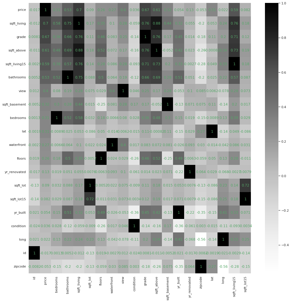
- Scikit - Learn 라이브러리
from sklearn.linear_model import LinearRegression

model = LinearRegression()
feature = ['sqft_living']
target = ['price']
X_train = df[feature]
y_train = df[target]
model.fit(X_train, y_train)
X_test = [[15000]]
y_pred = model.predict(X_test)

print(f'{X_test[0][0]} sqft living를 가지는 주택의 예상 가격은 ${y_pred} 입니다.')

# 15000 sqft living를 가지는 주택의 예상 가격은 $[[4165772.77536725]] 입니다.- 다중선형회귀 ( Multiple Linear Regression )
- 회귀모델을 평가하는 평가지표들 ( Evaluation Metrics )
- MSE ( Mean Squared Error ) : 전차 제곱의 합의 평균
- MAE ( Mean Absolute Error ) : 전차 절대값의 합
- RMSE ( Root Mean Squared Erroe ) : MSE의 루트를 씌운 값
- R - Squared ( Coefficient of Determination )
- 참고
- SSE ( Sum of Squared Error, 관측치와 예측치 차이 )
- SSR ( Sum of Squared due to Regression, 예측치와 평균 차이 )
- SST ( SUm of Squared Total, 관측치와 평균 차이 )
- 과적합 ( Overfitting ) : 과하게 학습해 일반화를 못해 결국 테스트 데이터에서 오차가 커지는 현상
ex) 분산이 높은 경우 - 과소적합 ( Underfitting ) : 과적합도 못하고 일반화 성질도 학습하지 못해 훈련 / 테스트 데이터 모두 오차가 크게나오는 경우
ex) 편향이 높은 경우 - 이상치 대체 및 제거 함수
def kill_outlayers(dataset,feature,processing_system):
  Q1 = dataset[feature].quantile(0.25)
  Q3 = dataset[feature].quantile(0.75)
  IQR = Q3 - Q1
  lower_limit = Q1 - 1.5*IQR
  upper_limit = Q3 + 1.5*IQR
  if processing_system == "mean" :
    processing_value = dataset[feature].mean
    for i in range(0,dataset.shape[0]) :
      if dataset.loc[i,f"{feature}"] > upper_limit :
          dataset.loc[i,f"{feature}"] =processing_value
      elif dataset.loc[i,f"{feature}"] < lower_limit :
         dataset.loc[i,f"{feature}"] =processing_value
      else :
        continue
  elif processing_system == "median" :
    processing_value = dataset[feature].median
    for i in range(0,dataset.shape[0]) :
      if dataset.loc[i,f"{feature}"] > upper_limit :
          dataset.loc[i,f"{feature}"] =processing_value
      elif dataset.loc[i,f"{feature}"] < lower_limit :
         dataset.loc[i,f"{feature}"] =processing_value
      else :
        continue
  elif processing_system == "drop" :
    indexs =[]
    for i in range(0,dataset.shape[0]) :
      if dataset.loc[i,f"{feature}"] > upper_limit :
          indexs.append(i)
      elif dataset.loc[i,f"{feature}"] < lower_limit :
          indexs.append(i)
      else :
        continue
    dataset.drop(dataset.index[indexs],inplace =True)
    dataset.reset_index(drop=True,inplace =True)
return dataset- 훈련 / 테스트 데이터셋 나누기
from sklearn.model_selection import train_test_split

x = df[['bathrooms', 'grade', 'sqft_living', 'sqft_living15', 'sqft_sum']]
y = df['price']
x_train, x_test, y_train, y_test = train_test_split(x, y, train_size=0.8, test_size=0.2)- 평가지표 함수
from sklearn.metrics import  mean_squared_error, mean_absolute_error, r2_score


def train_evaluation_metrics(y, y_pred):
  # 평가지표
  mse = mean_squared_error(y, y_pred)
  mae = mean_absolute_error(y, y_pred)
  rmse = mse ** 0.5
  r2 = r2_score(y, y_pred)
  print(f'훈련 MSE: {mse:.2f}')
  print(f'훈련 MAE: {mae:.2f}')
  print(f'훈련 RMSE: {rmse:.2f}')
  print(f'훈련 R2: {r2:.2f}')

def test_evaluation_metrics(y, y_pred):
  # 평가지표
  mse = mean_squared_error(y, y_pred)
  mae = mean_absolute_error(y, y_pred)
  rmse = mse ** 0.5
  r2 = r2_score(y, y_pred)
  print(f'테스트 MSE: {mse:.2f}')
  print(f'테스트 MAE: {mae:.2f}')
  print(f'테스트 RMSE: {rmse:.2f}')
  print(f'테스트 R2: {r2:.2f}')
train_evaluation_metrics(y_train, y_pred_1)
test_evaluation_metrics(y_test, y_pred_2)- 다중선형회귀
from sklearn.linear_model import LinearRegression

model = LinearRegression()

model.fit(x_train, y_train)

y_pred_1 = model.predict(x_train)
y_pred_2 = model.predict(x_test)- 원핫인코딩 ( One Hot Encoding ) : 범주형 변수를 변환
- Category_ecoders
from category_encoders import OneHotEncoder
encoder = OneHotEncoder(use_cat_names = True)
df_ohe = encoder.fit_transform(df)- 특성 선택 ( Feature Selection ) :
- Filter Method : Feature 간 관련성을 측정하는 방법
- Filter Method는 통계적 측정 방법을 사용하여 피처간의 상관관계를 알아낸 뒤,
- 높은 상관계수(영향력)를 가지는지 피처를 사용하는 방법입니다.
- 하지만, 상관계수가 높은 피처가 반드시 모델에 적합한 피처라고 할 수는 없습니다.
- Filter Method는 아래와 같은 방법이 존재합니다.
- information gain
- chi-square test
- fisher score
- correlation coefficient
- variance threshold
- Wrapper Method : Feature Subset의 유용성을 측정하는 방법
- Wrapper method는 예측 정확도 측면에서 가장 좋은 성능을 보이는 Feature subset(피처 집합)을 뽑아내는 방법입니다.
- 이 경우, 기존 데이터에서 테스트를 진행할 hold-out set을 따로 두어야하며,
- 여러번 Machine Learning을 진행하기 때문에 시간과 비용이 매우 높게 발생하지만
- 최종적으로 Best Feature Subset을 찾기 때문에, 모델의 성능을 위해서는 매우 바람직한 방법입니다.
- 물론, 해당 모델의 파라미터와 알고리즘 자체의 완성도가 높아야 제대로 된 Best Feature Subset을 찾을 수 있습니다.
- Wrapper Method는 아래와 같은 방법이 존재합니다.
- Forward Selection(전진 선택)
- Backward Elimination(후방 제거)
- Stepwise Selection(단계별 선택)
- Embedded Method : Feature Subset의 유용성을 측정하지만, 내장 metric을 사용하는 방법
- Embedded method는 Filtering과 Wrapper의 장점을 결함한 방법으로,
- 각각의 Feature를 직접 학습하며, 모델의 정확도에 기여하는 Feature를 선택합니다.
- 계수가 0이 아닌 Feature가 선택되어, 더 낮은 복잡성으로 모델을 훈련하며, 학습 절차를 최적화합니다.
- Embedded Method는 아래와 같은 방법이 존재합니다.
- LASSO : L1-norm을 통해 제약을 주는 방법, 연구자가 직접 판단 - 특성을 확인하고 없애 버린다.
- Ridge : L2-norm을 통해 제약을 주는 방법, 자동으로 특성 선별 후 불필요한 특성 제거
- Elastic Net : 위 둘을 선형결합한 방법
- SelectFromModel
- Filter Method : Feature 간 관련성을 측정하는 방법
from sklearn.feature_selection import f_regression, SelectKBest
from sklearn.linear_model import RidgeCV

selector = SelectKBest(score_func=f_regression, k=20)
X_train_selected2 = selector.fit_transform(X_train2, y_train2)
X_test_selected2 = selector.transform(X_test2)

alphas = [0, 0.001, 0.01, 0.1, 1, 10, 100, 1000]

ridge = RidgeCV(alphas=alphas,normalize=True, cv=5)
ridge.fit(X_train_selected2,y_train2)- 분류 평가지표
- Accuracy
- Logistic Regression
- Odds : 실패확률에 대한 성공확률의 비
- 중복 샘플 확인
df.duplicated()- 중복 샘플 제거
df.drop_duplicates(inplace = True)- 훈련 / 검증 / 테스트 분리
from sklearn.model_selection import train_test_split
train, test = train_test_split(df, train_size = 0.8, test_size = 0.2, random_state = 2)
train, val = train_test_split(train, train_size = 0.8, test_size = 0.2, random_state = 2)- 정확도
from sklearn.linear_model import LogisticRegression
logistic = LogisticRegression(max_iter=1000)
logistic.fit(X_train, y_train)

print('검증세트 정확도', logistic.score(X_val, y_val))- 타겟 데이터 분산 확인
submission.value_counts(normalize = True)import seaborn as sns
import matplotlib.pyplot as plt
%matplotlib inline
sns.countplot(x=y_pred_test)
- 분류 평가지표
- 모델의 예측값에 Threshold가 적용되어 최종적으로 분류된 결과를 평가하는 지표들입니다.
- Threshold가 바뀔 경우 평가 지표의 값도 바뀝니다.
- TP / TN / FP / FN
예측 1 예측 0 실제 1 TP FN 실제 0 FP TN - TP == True Positive == 진짜 양성 == 실제 1, 예측 1
- TN == True Negative == 진짜 음성 == 실제 0, 예측 0
- FP == False Positive == 가짜 양성 == 실제 0, 예측 1 == 모델이 가짜로 1이라고 한 것
- FN == False Negative == 가짜 음성 == 실제 1, 예측 0 == 모델이 가짜로 0이라고 한 것
- 결정트리 ( Decision Trees ) : 어떤 조건에 대해서 boolean으로 대답하는것
- 트리 학습 비용함수
- 지니불순도
- 엔트로피
- 파이프라인 사용
from ipywidgets import interact
from sklearn.metrics import f1_score
from sklearn.tree import DecisionTreeClassifier
from category_encoders import OneHotEncoder
from sklearn.impute import SimpleImputer
from sklearn.pipeline import make_pipeline

def thurber_tree(max_depth=1):
    pipe = make_pipeline(
    OneHotEncoder(use_cat_names=True),
    SimpleImputer(),
    DecisionTreeClassifier(max_depth = max_depth, random_state=2))
    pipe.fit(X_train, y_train)
    y_pred = pipe.predict(X_val)
    print('검증세트정확도: ', pipe.score(X_val, y_val))
    print('F1-score: ', f1_score(y_val, y_pred))

interact(thurber_tree, max_depth=(1,50,1));- 특성중요도 그래프
importances = pd.Series(model_dt.feature_importances_, encoded_columns)
plt.figure(figsize=(10,30))
importances.sort_values().plot.barh()
- 앙상블 방법 : 한 종류의 데이터로 여러 머신러닝 학습모델을 만들어 그 모델들의 예측결과를 다수결이나 평균을 내어 예측하는 방법
- Random Forests
- 버깅 ( Bagging , Bootstrap Aggregting ) : Bootstrap으로 훈련된 데이터를 다시 합치는 과정
- 부스스트랩 ( Bootstrap ) 샘플링 : 원본 데이터에서 샘플링을 하는데 복원추출을 한다는 것
from sklearn.impute import SimpleImputer
from sklearn.pipeline import make_pipeline
from sklearn.ensemble import RandomForestClassifier
from sklearn.metrics import f1_score

pipe_ord = make_pipeline(
    OrdinalEncoder(),
    SimpleImputer(),
    RandomForestClassifier(random_state=2, n_jobs=-1, oob_score=True)
)

pipe_ord.fit(X_train, y_train)
print('검증 정확도', pipe_ord.score(X_val, y_val))- 원핫인코딩 VS 순서형 인코딩
- OneHotEncoding : 카테고리 수에 따라 새로운 특성 생성 -> 카테고리가 많이 없고, 명목형 데이터 일 때
- OrdinalEncoding : 열 개수는 그대로 유지 ( 1개 ) 카테고리 별 중요도가 설정됨 -> 카테고리 별로 중요도가 다를 때
- Confusion Matrix
from sklearn.metrics import plot_confusion_matrix
import matplotlib.pyplot as plt

fig, ax = plt.subplots()
pcm = plot_confusion_matrix(pipe, X_val, y_val,
                            cmap=plt.cm.Purples,
                            ax=ax);
plt.title(f'Confusion matrix, n = {len(y_val)}', fontsize=15)
plt.show()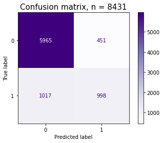
- 정밀도 ( Precision ) : Positive로 예측한 경우 중 올바르게 Positive를 맞춘 비율
- 재현율 ( Recall ) : 실제 Positive인 것 중 올바르게 Positive를 맞춘 비율
- F1-Score : 정밀도와 재현율의 조화평균이다.
- 임계값
from ipywidgets import interact, fixed
import seaborn as sns
import matplotlib.pyplot as plt
from sklearn.metrics import classification_report

def explore_threshold(y_true, y_pred_proba, threshold=0.5):
    y_pred = y_pred_proba >= threshold
    vc = pd.Series(y_pred).value_counts()
    ax = sns.histplot(y_pred_proba, kde=True)
    ax.axvline(threshold, color='red')
    ax.set_title(f'# of target, 1={vc[1]}, 0={vc[0]}')
    plt.show()
    print(classification_report(y_true, y_pred))


interact(explore_threshold,
    y_true=fixed(y_val),
    y_pred_proba=fixed(y_pred_proba),
    threshold=(0, 1, 0.01));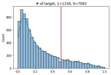
임계값에 따른 그래프
- ROC ( Receiver Operating Characteristic ) : 머신러닝의 이진 분류 모델의 예측 성능을 판단하는 중요한 평가지표
fpr, tpr, thresholds = roc_curve(y_val, y_pred_proba)

roc = pd.DataFrame({
    'FPR(Fall-out)': fpr,
    'TPRate(Recall)': tpr,
    'Threshold': thresholds
})
roc
plt.scatter(fpr, tpr)
plt.title('ROC curve')
plt.xlabel('FPR(Fall-out)')
plt.ylabel('TPR(Recall)');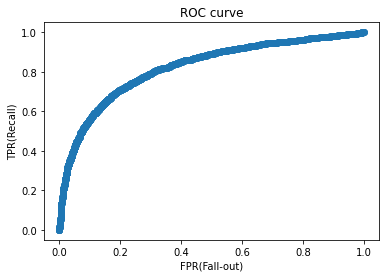
- AUC ( Area Under Curve ) : ROC 곡선 밑의 면적을 구한 것
from sklearn.metrics import roc_auc_score
auc_score = roc_auc_score(y_val, y_pred_proba)
auc_score- 교차검증 ( Cross - Validation )
- 시계열 ( Time Series ) 데이터에 적합하지 않음
- TargetEncoder
- OrdinalEncoder 보다 요즘 성능이 좋음.
- 하이퍼파라미터 튜닝
- 최적화 : 훈련 데이터로 더 좋은 성능을 얻기 위해 모델을 조정하는 과정
- 일반화 : 처음 본 데이터로 얼마나 좋은 성능을 내는지
- RandomizedSearchCV : 무작위
from sklearn.pipeline import make_pipeline
from category_encoders import OrdinalEncoder
from sklearn.impute import SimpleImputer
from sklearn.ensemble import RandomForestClassifier
from scipy.stats import randint, uniform
from sklearn.model_selection import RandomizedSearchCV


pipe = make_pipeline(
    OrdinalEncoder(),
    SimpleImputer(),
    RandomForestClassifier(random_state=2)
)

dists = {
    'simpleimputer__strategy': ['mean', 'median'],
    'randomforestclassifier__n_estimators': randint(50, 500),
    'randomforestclassifier__max_depth': [5, 10, 15, 20, None],
    'randomforestclassifier__max_features': uniform(0, 1) # max_features
}

clf = RandomizedSearchCV(
    pipe,
    param_distributions=dists,
    n_iter=20,
    cv=3,
    scoring='f1',
    verbose=1,
    n_jobs=-1
)

clf.fit(X_train, y_train)
print('최적 하이퍼파라미터: ', clf.best_params_)
- GridSearchCV : 전체
from category_encoders import TargetEncoder
from sklearn.model_selection import GridSearchCV

pipe = make_pipeline(
    TargetEncoder(),
    SimpleImputer(),
    RandomForestClassifier(random_state=2,class_weight='balanced')
)

dists = {
    'simpleimputer__strategy': ['mean', 'median'],
    'randomforestclassifier__n_estimators': [10, 50, 100],
    'randomforestclassifier__max_depth': [10, 50, 100],
    'randomforestclassifier__max_features': ['auto','log2'],
    'randomforestclassifier__min_samples_leaf' : [1, 3, 5]
}

clf = GridSearchCV(
    pipe,
    param_grid=dists,
    cv=3,
    scoring='f1',
    verbose=1,
    n_jobs=-1
)

clf.fit(X_train, y_train)
print('최적 하이퍼파라미터: ', clf.best_params_)- 특성 중요도 ( Feature Importances )
- 피쳐 중요도 ( Tree ) : 노드들의 지니불순도 / Information Gain을 기준으로 계산
- 장점 : 빠른 속도
- 단점 : Model-Dependent, High-Cardinality에 치우친 결과
- Drop-Column 중요도 : 각 특성들을 Drop하고 모델을 Re-Fit을 한후 Evaluate
- 장점 : 직관적
- 단점 : 매우 느림
- 순열 중요도 ( Permutation Importances ) : 각 특성들을 Shuffle하고 모델 Evaluate
- 장점 : Drop-Column 과 매커니즘을 비슷하면서도 속도가 빠름
- 단점 : 랜덤성
- 피쳐 중요도 ( Tree ) : 노드들의 지니불순도 / Information Gain을 기준으로 계산
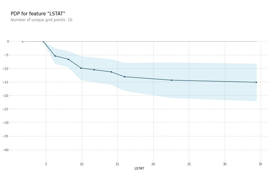
- PDP : 모델의 예측값이 특정 피쳐의 변화에 따라 평균적으로 어떻게 변하는지 보여주는 그래프
- ICE 곡선 : 특정 데이터에 대해 모델의 예측값이 특정 피쳐의 변화에 따라 어떻게 변하는지 보여주는 그래프
- 해석 시 유의할 점
- 각 변수들 분포의 독립성 가정
- 변수의 분포를 함께 고려할 것
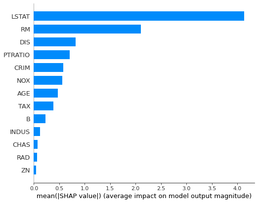
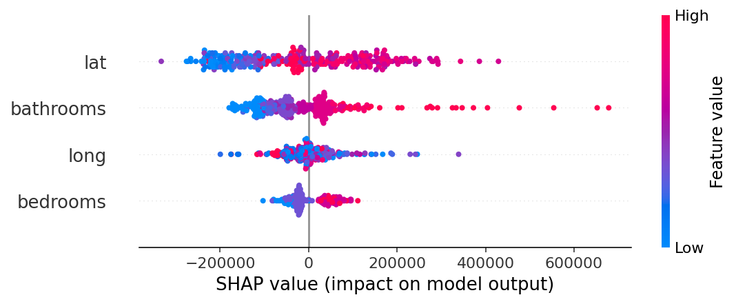
- SHAP : 특정 데이터에 대해 모델의 예측값에 각 피처들이 얼마나 기여했는지를 보여줌
728x90
반응형
'AI > Codestates' 카테고리의 다른 글
| [Day 46] SQL (01) (0) | 2022.03.29 |
|---|---|
| [Day 45] 개발환경 (0) | 2022.03.29 |
| [Day38 ~ Day43] Section 2 Project (0) | 2022.03.25 |
| [Day 37] Sprint Review (0) | 2022.03.25 |
| [Day 36] Interpreting ML Model (0) | 2022.03.25 |